Relational Algebra To SQL Translation.

Relational Algebra (RA) is the mathematical foundation of SQL. Understanding how to translate RA operations to SQL is crucial for query optimization, database design, and performance tuning. This guide covers all core RA operations, their SQL equivalents, and practical translation techniques.

What is Relational Algebra?

Relational Algebra is a formal system for manipulating relations (tables) in a relational database. It consists of a set of operations that take one or two relations as input and produce a new relation as output. The primary operations in relational algebra include:

• Selection (σ): Filters rows based on a specified condition.
• Projection (π): Selects specific columns from a relation.
• Union (∪): Combines the tuples of two relations, removing duplicates.
• Difference (−): Returns tuples that are in one relation but not in another.
• Cartesian Product (×): Combines every tuple of one relation with every tuple of another.
• Join (⨝): Combines tuples from two relations based on a related attribute.

Relational algebra provides a theoretical foundation for relational databases and is used to formally express queries.

What is SQL?

SQL (Structured Query Language) is a standard programming language used for managing and manipulating relational databases. It allows users to perform various operations such as querying data, updating records, inserting new data, and deleting existing data. SQL is widely used due to its simplicity and effectiveness in handling structured data.

Key components of SQL include:

• Data Query Language (DQL): Used for querying data (e.g., SELECT statements).
• Data Definition Language (DDL): Used for defining database structures (e.g., CREATE, ALTER, DROP).
• Data Manipulation Language (DML): Used for manipulating data (e.g., INSERT, UPDATE, DELETE).
• Data Control Language (DCL): Used for controlling access to data (e.g., GRANT, REVOKE).

Why is Translation Important?

The translation from Relational Algebra to SQL is important for several reasons:

1. Theoretical Foundation: Relational algebra provides a formal basis for understanding the operations that can be performed on relational data. SQL, being a practical implementation, is built upon these theoretical concepts.

2. Optimization: Understanding the relational algebra expressions allows database systems to optimize SQL queries. By translating SQL into relational algebra, the database engine can apply various optimization techniques to improve query performance.

3. Query Design: Knowledge of relational algebra helps database designers and developers to construct more efficient and effective SQL queries. It encourages a deeper understanding of how data is structured and accessed.

4. Interoperability: Many database systems support SQL, but the underlying principles of relational algebra remain consistent. This allows for easier migration and adaptation of queries across different systems.

5. Educational Value: Teaching relational algebra alongside SQL helps students and practitioners grasp the underlying principles of relational databases, leading to improved programming practices and more effective database design.

The translation from relational algebra to SQL bridges the gap between theoretical concepts and practical applications, enhancing both the performance and understanding of database operations.

How to Translate Relational Algebra to SQL?

Translating a relational algebra expression to an SQL query involves several steps. Here’s a structured approach to perform this translation, along with an example.

Steps to Translate Relational Algebra to SQL:

1. Identify the Relations: Determine the tables involved in the relational algebra expression.

2. Identify the Operations: Recognize the operations being performed (e.g., selection, projection, join, etc.).

3. Translate Selection (σ): Use the WHERE clause in SQL to filter rows based on the specified condition. Example:

• RA: σ_{Salary > 5000}(Employees)
• SQL: SELECT * FROM Employees WHERE Salary > 5000;

4. Translate Projection (π): Use the SELECT statement to specify the columns to be retrieved. Example:

• RA: π_{Name, Dept}(Employees)
• SQL: SELECT Name, Dept FROM Employees;

5. Translate Join (⨝): Use the JOIN clause to combine tables based on a related attribute. Example:

• RA: R ⋈ S (Natural Join)
• SQL: SELECT * FROM R JOIN S ON R.A = S.A;

6. Translate Union (∪): Use the UNION operator to combine results from two queries. Example:

• RA: Active_Employees ∪ Retired_Employees
• SQL: SELECT * FROM Active_Employees UNION SELECT * FROM Retired_Employees;

7. Translate Difference (−): Use a combination of SELECT and NOT IN or EXCEPT to find differences between two relations. Example: 

• RA: Students − Graduates
• SQL: SELECT * FROM Students EXCEPT SELECT * FROM Graduates;

8. Combine the Translations: Assemble the SQL query by combining the translated components in the correct order.

Example to Convert Relational Algebra to SQL Query:

Let's consider a simple example with two relations:

Students: Contains student information.

• Attributes: StudentID, Name, Major

Courses: Contains course information.

• Attributes: CourseID, CourseName, Instructor

Relational Algebra Expression

Suppose we want to find the names of students who are majoring in "Computer Science" and are enrolled in a course taught by "Dr. Smith". The relational algebra expression might look like this:

1. Selection: Select students majoring in "Computer Science".

$S1={\sigma }_{\text{Major}{=}^{\prime }ComputerScienc{e}^{\prime }}(\text{Students})$

2. Join: Join with the Courses table where the instructor is "Dr. Smith".

$S2=S1\bowtie {\sigma }_{\text{Instructor}{=}^{\prime }Dr.Smit{h}^{\prime }}(\text{Courses})$

3. Projection: Project the students' names.

${\pi }_{\text{Name}}(S2)$

Now, let's translate this into an SQL query:

SELECT s.Name
FROM Students s
JOIN Courses c ON s.StudentID = c.CourseID
WHERE s.Major = 'Computer Science' AND c.Instructor = 'Dr. Smith';

Explanation of the SQL Query

1. SELECT s.Name: This corresponds to the projection operation, where we want to retrieve the names of the students.

2. FROM Students s: This specifies the primary table (Students) and gives it an alias (s).

3. JOIN Courses c ON s.StudentID = c.CourseID: This represents the join operation, where we are joining the Students table with the Courses table based on a common attribute (assuming StudentID is related to CourseID for this example).

4. WHERE s.Major = 'Computer Science' AND c.Instructor = 'Dr. Smith': This corresponds to the selection operation, filtering the results to only include students majoring in "Computer Science" and enrolled in courses taught by "Dr. Smith".

By following these steps, you can systematically translate relational algebra expressions into SQL queries, ensuring that the logic and intent of the original query are preserved.

Data Models in DBMS.

Data Models in DBMS play an important role in organizing and managing data efficiently. A data model acts as a blueprint that defines how data is stored, connected, and accessed in a database. It bridges the gap between real-world information and how it is represented digitally, enabling better data management, consistency, and security.

What is a Data Model?

A Data Model in DBMS (Database Management System) is a conceptual framework that defines how data is structured, stored, connected, and manipulated within a database. It acts as a blueprint for building and organizing a database by providing rules and guidelines for how data should be represented.

Data models help users and developers understand the data and its relationships without worrying about how it is physically stored. They offer a high-level view of the data and ensure consistency, integrity, and clarity in database design. Data models also help in translating real-world scenarios into a structured database format.

Why Are Data Models Important in DBMS?

Data models are important because they help us organize data clearly and logically. They define how data is stored, related, and accessed, making it easier for developers, users, and database administrators to understand and manage the database. Without a data model, managing large amounts of data would be confusing and error-prone. A good data model ensures consistency, improves data quality, and supports better performance and scalability.

Key Purposes of a Data Model:

• It defines how data is stored, connected, and accessed.
• It helps in database design and communication among stakeholders.
• It enables data abstraction for various levels (user, logical, physical).
• It enhances data consistency, integrity, and security.

Types of Data Models in DBMS.

DBMS data models are broadly categorized into three main types:

• High-Level Data Models (Conceptual Models).
• Record-Based Data Models (Logical Models).
• Physical Data Models.

Let's discuss each of them one by one in complete detail with examples.

1️⃣ High-Level Data Models (Conceptual Models)

High-Level Data Models, also known as Conceptual Models, are used to describe what data is stored in the database and the relationships among those data without worrying about how the data is actually stored physically. These models focus on the meaning of the data and are often used during the initial design of a database.

They are easy to understand and help bridge the gap between technical database designers and non-technical stakeholders (like business users).

Key Characteristics:

• Focus on what data is needed, not how it is stored.
• Use simple diagrams to represent entities (like users or products) and their relationships.
• Hide low-level implementation details such as file formats or indexing.
• Often modeled using Entity-Relationship (ER) diagrams.

Example: 

Imagine you're designing a university database. In this case, the main entities would be Student, Course, and Instructor. The relationships between them could include a Student enrolling in multiple Courses and a Course being taught by one Instructor. 

These connections and entities are represented visually using an Entity-Relationship (ER) diagram, where rectangles denote entities, ovals represent attributes (such as student name or course name), and diamonds indicate relationships (like “enrolls in” or “teaches”). At this stage, the focus is on what data is important and how it logically connects, not on how it’s physically stored in the database.

2️⃣ Record-Based Data Models (Logical Models).

Record-Based Data Models, also known as Logical Data Models, describe how data is logically structured and how relationships between data are maintained. These models are called “record-based” because they represent data as fixed-format records of various types. Unlike conceptual models that focus on high-level design, logical models are more detailed and closer to how the data is actually stored in a database.

There are three main types of Record-Based Models:

• Relational Model
• Hierarchical Model
• Network Model

Let's discuss each of them in detail.

1. Relational Data Model: The relational model represents data in the form of tables (relations), where each table consists of rows (records) and columns (attributes). It uses primary keys and foreign keys to establish relationships between tables.

Example: Example: A customer table with customer details and an order table linked via customer ID.

2. Hierarchical Data Model: The hierarchical model organizes data in a tree-like structure with parent-child relationships. Each parent can have multiple children, but each child has only one parent. It is fast for read operations with a clear structure, but lacks flexibility for complex relationships.

Example: Example: An organization chart where a manager supervises multiple employees.

3. Network Data Model: This model represents data as a graph, allowing many-to-many relationships. It is more flexible than the hierarchical model, but can be complex to design and maintain.

Example: Students enrolled in multiple courses, and each course has multiple students.

3️⃣ Physical Data Model.

A Physical Data Model represents how data is actually stored in the computer system. It deals with the physical storage of data, including files, indexing, partitions, memory locations, and access paths. This model is closest to the hardware and focuses on optimizing performance, storage efficiency, and data retrieval speed.

While the Conceptual and Logical models focus on what data is stored and how it is logically related, the Physical Data Model focuses on how that data is actually written to disk and accessed efficiently.

Key Characteristics:

• Defines data storage structures like tables, indexes, and constraints.
• Specifies data types, column lengths, and storage format.
• Optimizes data access paths using techniques like indexing and clustering.
• Deals with database performance tuning, space allocation, and I/O optimization.

Example: In a physical data model, a Student table is stored on disk with an indexed StudentID and data types like VARCHAR(100) for names and INT for IDs to optimize storage and retrieval.

Which Model to Choose When?

Model	Best For	Avoid If
Relational	Structured data, complex queries	Unstructured data, high scalability
NoSQL	Big data, flexible schemas	ACID transactions, complex joins
Hierarchical	Tree-like data (e.g., file systems)	Many-to-many relationships
Network	Graph data (rarely used today)	Modern applications
Object-Oriented	OOP systems, multimedia data	High-performance needs

Final Recommendation:

• Use Relational for transactional systems (banking).
• Use NoSQL for scalability (social media, IoT).
• Use Hierarchical/Network only for legacy systems.

FAQs on Data Models in DBMS

Q1: Which is the most widely used data model in DBMS?

➡️ The Relational Model is the most commonly used due to its simplicity and support by modern RDBMS like MySQL and SQL Server.

Q2: What is the purpose of a conceptual data model?

➡️ It provides a high-level view of data for users and stakeholders, hiding implementation details.

Q3: Can a DBMS support multiple data models?

➡️ Yes, modern DBMS can support hybrid models like document and relational (e.g., PostgreSQL, MongoDB).

Conclusion.

Data models are the backbone of any database system. From high-level designs to physical storage, they provide structure, clarity, and flexibility. Whether you're designing a simple database or a large-scale system, understanding these models is key to efficient, scalable, and secure database development.

Relational Integrity Constraints

In a Relational Database Management System (RDBMS), integrity constraints are rules that enforce data accuracy, consistency, and reliability. These constraints ensure that the database remains error-free, even when multiple users insert, update, or delete data.

Without integrity constraints, databases could suffer from:

❌ Duplicate records

❌ Invalid relationships (e.g., an order without a customer)

❌ Inconsistent data (e.g., negative age values)

In this article, we’ll explore the types of relational integrity constraints, their importance, and real-world examples.

Before reading this article, you should read the following DBMS topics:

• DBMS Introduction.
• Data Models in DBMS.
• Types of Keys in DBMS.

What are Relational Integrity Constraints?

Relational Integrity Constraints are rules that ensure data in a database remains accurate, consistent, and reliable. They prevent invalid entries, broken relationships, or illogical data by enforcing conditions on tables, columns, and relationships.

For example, a primary key ensures each row is unique, a foreign key guarantees valid links between tables, and a check constraint blocks impossible values (like negative ages). These constraints act as "guardrails" to maintain data quality, whether during insertions, updates, or deletions.

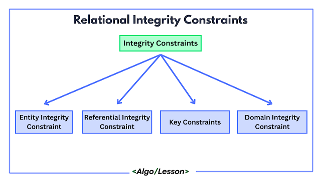
Types of Relational Integrity Constraints.

There are four types of Relational Integrity Constraints in DBMS:

• Entity Integrity Constraint.
• Referential Integrity Constraint.
• Domain Integrity Constraint.
• Key Constraints (Uniqueness).

1. Entity Integrity Constraint.

Entity Integrity Constraint ensures that each row in a table is uniquely identifiable and never left empty. 

It enforces two key rules:

• Primary Key (PK) must be unique (no duplicate values).
• PK cannot be NULL (every row must have an identifier).

This constraint guarantees that every record in a table can be distinctly accessed and referenced, preventing data ambiguity.

Example: Consider an example of the Employees Table with three columns.

Employee_ID (PK)	Name	Department
101	Alice	HR
102	Bob	IT
103	Charlie	Finance

How Entity Integrity Works:

Every Employee_ID (PK) must be unique and non-NULL in the Employees table.

✅ Valid: Employee_ID 103 (Charlie) is unique and not empty

❌ Invalid:
- Duplicate ID (101 for two employees)
- NULL value in Employee_ID

2. Referential Integrity Constraint.

Referential Integrity Constraint ensures that relationships between tables remain valid by enforcing that any value in a foreign key (FK) column must match an existing primary key (PK) value in the referenced table or be NULL. This prevents orphaned records (e.g., an order linked to a non-existent customer) and maintains data consistency across related tables.

Key Points:

• Ensures only valid relationships exist (e.g., no "ghost" customers for orders).
• Use ON DELETE CASCADE to auto-delete child records when a parent is removed.
• Blocks insertions/updates that break table relationships.

Example: Consider a relation between the parent (Customer) and child (Order) tables.

Customers (Parent Table)

Customer_ID (PK)	Name
1	Alice
2	Bob

Orders (Child Table)

Order_ID	Customer_ID (FK)	Amount
101	1	99.99
102	2	50.00

How Referential Integrity Works:

Every Customer_ID in the Orders table must exist in the Customers table's Customer_ID column.

✅ Valid: Order 101 links to Customer 1 (Alice)

❌ Invalid: An order with Customer_ID=3 would be rejected (no such customer exists)

3. Domain Integrity Constraint.

Domain Integrity Constraint ensures that all values in a database column adhere to defined rules, such as data types, formats, ranges, or custom conditions. It restricts what data can be entered into a column, preventing invalid or illogical values.

Key Aspects of Domain Integrity

• Data Type Enforcement: Columns must contain values of a specific type (e.g., INT, VARCHAR, DATE).
• Value Range/Rules: Uses CHECK constraints to limit values (e.g., Age >= 18).
• Mandatory Fields: NOT NULL ensures critical columns are never empty.
• Default Values: DEFAULT provides fallback values if none are specified.

Example: Employee Table with Domain Constraints

Employee_ID (INT PRIMARY KEY)	Name (VARCHAR(50) NOT NULL)	Age (INT CHECK >=18 AND <=70)	Email (VARCHAR(100) UNIQUE)	Join_Date (DATE DEFAULT CURRENT_DATE)	Salary (DECIMAL(10,2) CHECK >0)
101	Alice	30	alice@example.com	2023-10-05	5000.00

How Domain Integrity Works:

Each column enforces specific data rules:

✅ Valid Example: All values meet their constraints

❌ Violation Examples:

• NULL Name: (102, NULL, 25, 'bob@example.com', '2023-10-06', 4500.00)
• Age < 18: (103, 'Charlie', 17, 'charlie@example.com', '2023-10-07', 3000.00)
• Duplicate Email/Negative Salary: (104, 'Dave', 45, 'alice@example.com', '2023-10-08', -2000.00)

Key Constraints Shown:

• NOT NULL - Required fields
• CHECK - Value range validation
• UNIQUE - No duplicate emails
• DEFAULT - Automatic current date

4. Key Constraints (Uniqueness).

Key Constraints (Uniqueness) in database management systems enforce the principle that certain columns or combinations of columns must contain unique values across all rows in a table. These constraints are fundamental for maintaining data integrity by preventing duplicate entries in critical fields. 

The two primary types of uniqueness constraints are primary keys and unique keys, each serving distinct but related purposes. A primary key represents the main unique identifier for each record, requiring both uniqueness and non-null values, while a unique key also mandates distinct values but typically allows for one null entry. These constraints are implemented through database declarations that create automatic checks during data insertion or modification, rejecting any operation that would violate the uniqueness rule.

Example: Employee Table Example

CREATE TABLE Employees (
    Employee_ID INT PRIMARY KEY,         -- Primary Key (Unique + NOT NULL)
    Email VARCHAR(100) UNIQUE NOT NULL,  -- Unique Key (No duplicates)
    Passport_Number VARCHAR(20) UNIQUE   -- Unique Key (Allows one NULL)
);

Employee_ID (PK)	Email (Unique)	Passport_Number (Unique)
101	alice@company.com	A12345678
102	bob@company.com	B87654321
103	charlie@company.com	NULL
104	dave@company.com	C55555555

Key Observations:

• The Employee_ID column is the primary key - all values are unique and non-null
• The Email column has a unique constraint - no duplicates allowed (and NOT NULL enforced)
• The Passport_Number column has a unique constraint, but allows one NULL value

Conclusion.

Relational integrity constraints are essential for maintaining accurate, consistent, and reliable databases. By implementing PKs, FKs, CHECK, and UNIQUE constraints, you ensure data quality while improving performance.

Types of Keys in DBMS.

In Database Management Systems (DBMS), keys are the backbone of data organization, retrieval, and relationship management. They ensure that databases remain structured, efficient, and free from redundancy. Whether you're a beginner learning SQL or an experienced developer optimizing a database, understanding the different types of keys in DBMS is crucial for designing robust and scalable systems.

Keys serve multiple purposes:

• Uniquely identifying records (e.g., a student ID in a university database).
• Establishing relationships between tables (e.g., linking orders to customers).
• Maintaining data integrity by preventing duplicate or inconsistent entries.

In this article, we’ll explore the various types of keys in DBMS, their roles, and real-world use cases.

Types of Keys in the Relational Model.

Here is the list of Keys that are present in the Relational Model:

• Primary Key (PK) – Uniquely identifies each row (e.g., Student_ID).
• Foreign Key (FK) – Links tables by referencing a PK (e.g., Order.Customer_ID).
• Candidate Key – A potential PK (e.g., Email if unique).
• Alternate Key – Unused candidate keys (e.g., SSN when ID is PK).
• Composite Key – A PK made of multiple columns (e.g., (Student_ID, Course_ID)).
• Super Key – A set of columns containing a candidate key (e.g., {ID, Name}).

Let's discuss each of them one by one in detail,

1. Primary Key (PK).

A Primary Key (PK) is a column (or set of columns) in a table that uniquely identifies each row. It enforces data integrity by ensuring:

• No duplicate values (all entries must be unique).
• No NULL values (every row must have a PK value).

Key Features

• Uniqueness: Guarantees no two rows have the same PK value. Example: Employee_ID in the Employees table.
• Irreducibility: Cannot remove any column from a composite PK without breaking uniqueness.
• Mandatory: Every table must have exactly one PK (but can have multiple candidate keys).

Example:

CREATE TABLE Students (
    Student_ID INT PRIMARY KEY,  -- PK column
    Name VARCHAR(50),
    Email VARCHAR(100) UNIQUE    -- Candidate key
);

When to use Primary Key (PK)?

Use the Primary Key when:

• You need to uniquely identify each row in a table, such as assigning a unique EmployeeID to every record in an Employees table.
• You want to enforce data integrity, ensuring no duplicate or NULL values exist in the key column (e.g., ProductID in a Products table).
• Creating relationships between tables, as it serves as the target for Foreign Keys in related tables (e.g., CustomerID in a Customers table referenced by Orders).
• Optimizing query performance, since databases automatically index PKs for faster searches and joins (e.g., filtering orders by OrderID).
• Working with frameworks or ORMs, as most require a PK for CRUD operations (e.g., Django models or SQLAlchemy).

2. Foreign Key (FK).

A Foreign Key (FK) is a column (or set of columns) in a table that references the Primary Key (PK) of another table. It enforces referential integrity, ensuring valid relationships between tables.

Key Properties

• Links Tables: Creates relationships (e.g., Orders.Customer_ID → Customers.Customer_ID).
• Allows NULLs: Optional relationships (unless constrained).
• Supports Cascading Actions: Automatic updates/deletes (e.g., ON DELETE CASCADE).

Example:

CREATE TABLE Orders (
    Order_ID INT PRIMARY KEY,
    Customer_ID INT REFERENCES Customers(Customer_ID)  -- FK
);

When to use a Foreign Key (FK)?

Use a Foreign Key when:

• You need to link two tables, such as connecting an Orders table to a Customers table via CustomerID.
• You want to enforce referential integrity, ensuring that every record in the child table (e.g., Orders) corresponds to a valid record in the parent table (e.g., Customers).
• You want to automate updates or deletions across related tables, such as deleting all orders when a customer is removed (using ON DELETE CASCADE).
• Modeling relationships like one-to-many (e.g., one customer can have many orders) or many-to-one (e.g., many orders belong to one customer).

3. Candidate Key.

A Candidate Key is a minimal set of columns in a table that can uniquely identify each row without any redundancy. It satisfies two critical properties:

• Uniqueness: No two rows can have identical values in the candidate key columns.
• Irreducibility: No subset of the key can uniquely identify rows (it's "minimal").

Key Features

• A table can have multiple candidate keys.
• One candidate key is chosen as the Primary Key (PK); others become Alternate Keys.
• Candidate Key cannot contain NULL values (to ensure row uniqueness).

Example

In a Students table:

• Student_ID (Unique) → Candidate Key
• Email (Unique) → Candidate Key
• {Name, Birthdate} (If unique) → Composite Candidate Key

Note: All Primary Keys are candidate keys, but not all candidate keys become Primary Keys!

4. Alternate Key.

An Alternate Key is a candidate key that is not selected as the Primary Key (PK) in a table. It retains all properties of a candidate key (uniqueness and minimality) but serves as a backup unique identifier.

Key Features

• Uniqueness: Guarantees no duplicate values in its columns.
• Non-NULL: Cannot contain NULL values (like all candidate keys).
• Secondary Role: Used when the PK is impractical for certain queries.

Example

In a Students table:

• Primary Key (PK): Student_ID
• Alternate Keys: Email or SSN (if both are unique and minimal).

CREATE TABLE Students (
    Student_ID INT PRIMARY KEY,  
    Email VARCHAR(100) UNIQUE NOT NULL,  -- Alternate Key  
    SSN CHAR(9) UNIQUE NOT NULL          -- Alternate Key  
);

Note: Alternate Keys are implicitly indexed in most databases, just like PKs!

5. Composite Key.

A Composite Key is a type of primary key that consists of two or more columns that together uniquely identify each row in a table. The individual columns may contain duplicate values, but their combination must be unique.

Key Characteristics:

• Multi-Column Uniqueness: The combination of columns must be unique.
• Mandatory Fields: None of the component columns can contain NULL values.
• Relationship Enforcement: Often used in junction tables for many-to-many relationships.

Example:

In an Order_Details table that links orders to products:

CREATE TABLE Order_Details (
    OrderID INT NOT NULL,
    ProductID INT NOT NULL,
    Quantity INT,
    PRIMARY KEY (OrderID, ProductID)  -- Composite Key
);

When to use a Composite Key?

• When you need to uniquely identify relationships between entities
• When a single column isn't sufficient for uniqueness (e.g., flight number + date)
• When you need to uniquely identify records across multiple dimensions

6. Super Key.

A Super Key is any combination of columns in a table that can uniquely identify each row. Unlike candidate keys, super keys may contain extra columns that aren't strictly necessary for uniqueness.

Key Characteristics:

• Uniqueness Guarantee: Must uniquely identify each record.
• Non-Minimal: May include additional columns beyond what's needed for uniqueness.
• Flexible Composition: Can be any size from one column to all columns in the table.

In a Students table with columns:

• Student_ID (unique)
• Email (unique)
• Name
• Birthdate

Possible super keys include:

• {Student_ID}
• {Email}
• {Student_ID, Name}
• {Email, Birthdate}
• {Student_ID, Name, Email, Birthdate}

Conclusion.

Keys ensure data integrity, efficient querying, and logical relationships between tables. From Primary Keys that uniquely identify records to Foreign Keys that link tables, each key type serves a distinct purpose. Candidate Keys offer alternative unique identifiers, while Composite Keys handle complex relationships. Super Keys provide flexibility in uniqueness, and Alternate Keys act as backup identifiers.

Understanding these keys helps in:

✔ Designing optimized and scalable databases

✔ Maintaining data accuracy through constraints

✔ Improving query performance with proper indexing

Codd's 12 Rules for Relational Databases.

When E.F. Codd introduced the Relational Model in 1970, he also defined a set of 12 rules (numbered 0 to 12) that any Relational Database Management System (RDBMS) must satisfy to be considered truly relational. These rules serve as the foundation of relational databases, ensuring data integrity, independence, and consistency across systems.

Codd's Rules in DBMS.

Let’s explore each rule in simple words with examples.

Rule 0 – Foundation Rule.

"For a system to be considered relational, it must use its relational capabilities exclusively to manage the database."

Explanation: This is the baseline rule. It means the system must fully support all relational principles to qualify as a true RDBMS. Partial implementation (e.g., supporting SQL but not integrity rules) isn't enough.

Rule 1 – The Information Rule.

"All information in a relational database is represented explicitly at the logical level and in exactly one way – by values in tables."

Explanation: Every piece of data, including table names, column names, and actual data, should be stored in rows and columns. No hidden data, no pointers.

Example: A student’s name, age, and ID are stored in a Students table, not embedded in application logic.

Rule 2 – Guaranteed Access Rule.

"Each data item must be logically accessible by using a combination of table name, primary key, and column name."

Explanation: You should be able to retrieve any value in the database using a simple query, without needing to know the underlying storage structure.

Example: To get a student's name:

SQL Query: SELECT Name FROM Students WHERE StudentID = 101;

Rule 3 – Systematic Treatment of Null Values.

"Null values (distinct from zero or empty string) are supported for representing missing or inapplicable information."

Explanation: Nulls must be consistently treated and distinguishable from other values. They represent unknown or not applicable data.

Example: If a professor doesn't have an office assigned yet, the Office field should be NULL.

Rule 4 – Active Online Catalog (Data Dictionary)

"The database description is represented at the logical level in the same way as ordinary data, so authorized users can use the same relational language to access it."

Explanation: Metadata (like schema, tables, and columns) should be stored in tables and be queryable.

Example: This returns a list of tables in many RDBMS systems.

SQL Query: SELECT * FROM INFORMATION_SCHEMA.TABLES;

Rule 5 – Comprehensive Data Sub-language Rule.

"A relational system may support several languages and various modes of terminal use. But there must be one well-defined language that supports all of the following: data definition, data manipulation, data integrity constraints, and transaction control."

Explanation: There should be one powerful language (like SQL) that can handle everything: DDL, DML, constraints, and transactions.

Rule 6 – View Updating Rule

"All views that are theoretically updatable must be updatable through the system."

Explanation: If it’s logically possible to update a view, the system should allow it.

Example:

CREATE VIEW StudentNames AS SELECT Name FROM Students;
UPDATE StudentNames SET Name = 'Jane' WHERE Name = 'Janet';

Note: Not all views are updateable (e.g., ones with JOIN, GROUP BY, etc.).

Rule 7 – High-level Insert, Update, and Delete

"The system must support set-level inserts, updates, and deletes."

Explanation: You should be able to perform operations on multiple rows at once, not just one record at a time.

Example:

UPDATE Employees SET Bonus = 1000 WHERE Department = 'Sales';

Rule 8 – Physical Data Independence

"Changes to the physical storage of data should not require changes to applications that access that data."

Explanation: If you move your database from HDD to SSD or change the indexing method, your SQL queries should still work the same way.

Rule 9 – Logical Data Independence

"Changes to the logical structure (tables, views) should not affect how users interact with data."

Explanation: Applications should continue working even if the logical layout of data is modified.

Example: Splitting one large Employee table into CurrentEmployee and FormerEmployee shouldn’t break your application if views are maintained properly.

Rule 10 – Integrity Independence

"Integrity constraints must be stored in the catalog and not in application code."

Explanation: Rules like PRIMARY KEY, FOREIGN KEY, and CHECK constraints should be enforced by the database, not external applications.

Rule 11 – Distribution Independence

"The user should not be aware of whether the database is distributed."

Explanation: Whether your data is stored in one server or spread across many locations (distributed DB), it should be transparent to users.

Rule 12 – Non-subversion Rule

"If a system provides low-level access, it should not bypass the integrity rules or constraints."

Explanation: Even if there’s a “back door” or admin-level access, it must not allow data corruption or constraint violations.

Codd’s 12 Rules were visionary guidelines that laid the groundwork for modern relational databases. While few systems meet all of them perfectly, most modern RDBMSs strive to comply with them as much as possible to ensure scalability, security, and data integrity.

Relational Model in DBMS.

The Relational Model is the most widely used data model in database systems today. It organizes data into tables (called relations) that consist of rows (tuples) and columns (attributes). Each table represents a real-world entity, and each row represents a unique instance of that entity.

Developed by E.F. Codd in 1970, the relational model revolutionized data storage and management by using mathematical concepts from set theory and predicate logic. It provides a simple, intuitive, and flexible structure for handling structured data and enables powerful query capabilities using Structured Query Language (SQL).

What is the Relational Model?

The Relational Model is a fundamental data model in database management systems (DBMS) that represents data in the form of tables (called relations). Each table consists of rows (also called tuples) and columns (also called attributes).

The relational model is based on set theory and uses Structured Query Language (SQL) for data manipulation.

Key Features of the Relational Model:

• Data is organized into tables, each representing a real-world entity.
• Each row (tuple) in the table is a unique record.
• Each column (attribute) describes a property of the entity.
• Ensures data consistency, integrity, and independence.
• Enables powerful querying capabilities using SQL.

Example: The Relational Model represents data in tabular form, where:

• Table (Relation) → Collection of related data (e.g., Students table).
• Row (Tuple) → A single record (e.g., a student’s details).
• Column (Attribute) → A field representing a data type (e.g., Student_ID, Name).

Student_ID	Name	Age	Department
101	Alice	20	CS
102	Bob	22	EE

Key Concept of Relational Model.

The relational model is built on fundamental concepts that ensure data is organized, accessible, and maintainable. Here's a detailed explanation of each key concept with examples:

1. Relation (Table).

A relation is a two-dimensional table that organizes data about a specific entity. It consists of rows (tuples) and columns (attributes) that follow strict structural rules:

• Each relation has a unique name within the database
• All values in a column are from the same domain
• The order of rows and columns is insignificant
• No duplicate rows are allowed

2. Tuple (Row)

A tuple represents a single, complete record in a relation. Each tuple contains:

• An ordered set of attribute values
• A complete set of facts about one instance of an entity
• A unique identification through the primary key

Example: The tuple (101, 'Alice', 20, 'CS') represents all information about one specific student.

3. Attribute (Column/Field)

An attribute is a named column that represents a specific characteristic or property of the entity being modeled. Each attribute has:

• A name that is unique within its relation
• A defined data type and domain
• Optional constraints (NOT NULL, UNIQUE, etc.)

Example: In the STUDENTS relation, Student_ID, Name, Age, Department, etc, are attributes.

4. Domain

A domain defines the complete set of possible values that an attribute can take. It specifies:

• The data type (integer, string, date, etc.)
• Value constraints (range, format, etc.)
• Semantic meaning of the data

Example: For the Age attribute:

• Data type: INTEGER
• Valid range: 17 to 100
• NULL allowed: No
• Meaning: Current age in years

5. Degree

The degree of a relation refers to the number of attributes (columns) it contains. It indicates:

• How many different properties are recorded for each entity
• The complexity of the information stored

Example: The STUDENTS relation with 4 attributes (Student_ID, Name, Age, Department) has degree 4.

6. Cardinality

Cardinality refers to the number of tuples (rows) in a relation at any given time. It:

• Changes as data is inserted or deleted
• Indicates the size of the data set
• Affects query performance

Example: If the STUDENTS table contains 500 records, its current cardinality is 500.

7. Super Key

A super key is any set of attributes that can uniquely identify a tuple. It may contain extra attributes beyond what's strictly needed for uniqueness.

Example: In STUDENTS, {Student_ID}, {Student_ID, Name}, and {Name, Age, Department} (assuming unique) are all super keys.

8. Candidate Key

A candidate key is a minimal set of attributes (columns) in a relation (table) that can uniquely identify each tuple (row). It satisfies two critical properties:

• Uniqueness: No two tuples can have the same values for all attributes in the key.
• Irreducibility (Minimality): No proper subset of the key can uniquely identify tuples.

Key Characteristics

• A relation can have multiple candidate keys.
• One candidate key is chosen as the primary key.
• The remaining candidate keys become alternate keys.
• Candidate keys cannot contain NULL values (entity integrity rule).

Example: Student_ID and Email (if present and unique) could be candidate keys.

9. Primary Key

The primary key is the candidate key chosen by the database designer to be the main identifier for tuples in the relation.

Example: Student_ID is typically chosen as the primary key in the STUDENTS relation.

10. Alternate Key

An alternate key is any candidate key that was not selected as the primary key. These still provide a unique identification capability.

Example: If Email is a candidate key but not chosen as the primary key, it becomes an alternate key.

11. Foreign Key

A foreign key is an attribute (or set) in one relation that references the primary key of another relation, establishing a relationship between tables.

Example: In a COURSES table, Student_ID would be a foreign key referencing the STUDENTS table.

12. Composite Key

A composite key is a primary key that consists of two or more attributes, used when no single attribute can uniquely identify tuples.

Example: In a STUDENT_COURSES table tracking enrollments, the combination of Student_ID and Course_ID would form a composite primary key.

Comparison of Database Key Types

Key Type	Uniqueness	Minimality	NULL Allowed?	Purpose
Super Key	Yes	No	No	Any set that includes a candidate key.
Candidate Key	Yes	Yes	No	Potential primary keys.
Primary Key	Yes	Yes	No	The chosen main identifier.

13. Schema.

A schema is the structural definition of a database. It represents the logical design that remains constant unless modified intentionally.

Example Schema Definition (SQL):

14. Instance.

An instance (or database state) is the collection of data stored in the database at a particular moment. It is also called the "extension" of the database.

Example:

Advantages of the Relational Model.

• Simple tabular structure (easy to understand).
• Strong data integrity (PK, FK, constraints).
• Powerful querying with SQL.
• ACID compliance for reliable transactions.
• Reduced redundancy via normalization.

Disadvantages of the Relational Model.

• Slow for complex joins on large datasets.
• Inflexible schema (hard to modify).
• Struggles with unstructured data (JSON, graphs).
• Horizontal scaling challenges.
• Overhead for simple operations.

The Relational Model organizes data into tables with rows and columns, using keys to maintain relationships. It powers SQL-based databases like MySQL, PostgreSQL, and Oracle, making it the most widely used DBMS model today.

Developed by Edgar F. Codd, also gave us 12 rules to follow to make a database truly "relational." While no commercial database fully satisfies all rules, they remain the gold standard for relational design.

Generalization, Specialization and Aggregation in ER Model.

Designing a large and complex database using the ER (Entity-Relationship) model can quickly become overwhelming. The concepts of Generalization, Specialization, and Aggregation were introduced to address this challenge and simplify database design. These techniques provide powerful abstraction mechanisms that help hide unnecessary details while emphasizing important relationships and hierarchies within the data. 

In this article, we’ll explore these three key ER model components, understand how they work, and see real-world examples that demonstrate their practical use in database design.

What is Generalization in the ER Model?

Generalization is a process in the ER model where two or more lower-level entities are combined to form a higher-level, more general entity. It is a bottom-up approach in database design, where common features or attributes from multiple entities are grouped into a single generalized entity to reduce redundancy and improve clarity.

This abstraction helps simplify complex data structures by identifying shared characteristics among different entities and combining them under a unified parent entity.

Characteristics of Generalization.

• It follows a bottom-up approach, combining similar lower-level entities into a higher-level entity.
• Represents an "is-a" relationship (e.g., Car is a Vehicle).
• Common attributes are promoted to the generalized entity to avoid duplication.
• Helps in data abstraction and simplifies the ER model.
• Represented in ER diagrams using a triangle pointing to the general entity.

Generalization Example:

• In a university database, we may initially define two separate entities: Student and Teacher. Each entity has its own set of attributes. For example, a Student has attributes like StudentID, Name, and Email, while a Teacher has TeacherID, Name, and Email.
• Upon closer inspection, we notice that both entities share common attributes, specifically Name and Email. Instead of repeating these attributes in both entities, we can simplify our design through Generalization.
• We introduce a more generic entity called Person, which contains the common attributes: PersonID, Name, and Email. This entity acts as a superclass, or generalized entity, representing anyone in the system, whether a student or a teacher.
• Now, the original entities Student and Teacher become subclasses of Person. The Student entity adds specific attributes like CourseEnrolled, while the Teacher entity includes attributes like Department or SubjectTaught.

By using generalization, we reduce redundancy, improve clarity, and make our ER diagram cleaner and more scalable, especially useful in large, complex databases.

What is Specialization in ER Model?

Specialization is a concept in the Entity-Relationship (ER) model that allows you to break down a general entity into more specific sub-entities based on unique characteristics or roles. It is a top-down approach where you start from a broad, general entity set and create more detailed and refined entity sets. This is useful when some entities in a group need to be treated differently or have additional data.

Characteristics of Specialization.

• It follows an "is-a" relationship (e.g., a Manager is an Employee).
• Subclasses inherit attributes from the parent class.
• Can be disjoint (one entity belongs to only one subclass) or overlapping (an entity can belong to multiple subclasses).
• Helps in modeling real-world hierarchies and complex relationships.

Specialization Example.

Consider a general entity called Employee in a company database. All employees have common attributes like:

• EmployeeID
• Name
• Department
• Salary

But some employees might be Managers, and others might be Engineers:

• Managers may have TeamSize and DepartmentBudget attributes.
• Engineers may have ProjectAssigned and SkillSet attributes.

In this case:

• Employee is the superclass (general entity).
• Manager and Engineer are specialized subclasses.

This structure allows the system to store shared information in the Employee entity, while still capturing the unique aspects of each specialized role.

What is Aggregation in ER Model?

Aggregation is a concept in database management systems (DBMS) that allows you to treat a relationship between entities as a higher-level entity. It is a type of abstraction used in Entity-Relationship (ER) modeling to represent relationships involving multiple entities as a single unit.

Aggregation is particularly useful when:

• A relationship itself needs to participate in another relationship.
• You need to group entities and their relationships for better modeling.

Aggregation Example.

Consider a scenario where Employees work on Projects using Tools.

The relationship "Works_On" between Employee and Project needs to be linked with Tool to track which tools are used for which work.

Without Aggregation: You might struggle to directly relate the Tool to the Employee-Project relationship.

With Aggregation:

Entities:

• Employee (EmpID, Name)
• Project (ProjID, Title)
• Tool (ToolID, Name)

Relationship:

• Works_On (Employee ↔ Project)

Aggregation:

• The Works_On relationship is aggregated into a higher-level entity (e.g., Work).

Now, Tool can be linked to Work via a new relationship, Uses.

When to Use Aggregation?

• When a relationship needs to participate in another relationship.
• To simplify complex relationships in ER modeling.
• In scenarios like "a team (aggregation of employees) assigned to a project".

Aggregation helps in better database design by allowing relationships to be treated as entities when needed.

Entity-Relationship (ER) Model.

The Entity-Relationship (ER) Model is one of database design's most important and widely used conceptual data models. It helps developers and database designers visually represent the structure of a database in terms of entities, attributes, and relationships. The ER Model is crucial in simplifying complex data and transforming user requirements into a clear database structure.

What is ER Model in DBMS?

The Entity-Relationship (ER) Model is a way to visually design and organize a database. It shows the real-world objects (called entities), the details about those objects (called attributes), and the connections between them (called relationships). This model helps us understand how data is structured before actually building the database.

For example, in a school system, students, teachers, and courses are entities. A student can enroll in courses, and a teacher can teach courses. The ER model represents all this clearly in a diagram, making it easier to create and manage the database later.

Why Use ER Model in DBMS?

The ER (Entity-Relationship) Model is used in DBMS because it provides a clear and visual way to design the structure of a database before implementation. It helps developers and stakeholders understand the data requirements, relationships between entities, and business rules in a simple and intuitive format.

Using an ER model improves communication, reduces design errors, and ensures the database meets the real-world needs of the application. It also lays the foundation for creating normalized tables and writing efficient queries.

Key Benefits of Using ER Model:

• Simplifies database design through clear visuals of entities and relationships.
• Improves communication between developers and non-technical stakeholders.
• Reduces design errors by identifying relationships and constraints early.
• Supports normalization by helping spot redundant or misplaced data.
• Acts as a blueprint for converting to relational tables in RDBMS.
• Saves time and effort during later development phases.

Key Components of ER Model.

The ER Model consists of several key components that help structure and design a database logically. Each component plays a specific role in defining how data is stored and how different entities interact with each other.

1. Entity
Definition: An entity is a real-world object or thing that can be identified in the database.
Example: In a university system, Student, Course, and Professor are entities.

2. Entity Set
Definition: A collection of similar types of entities is called an Entity Set.
Example: All students in a university form a Student entity set.

3. Attributes
Definition: Attributes are properties or characteristics of an entity.
Example: A Student entity might have attributes like StudentID, Name, Email, and DateOfBirth.

4. Primary Key
Definition: Primary Key is a unique attribute (or combination) that identifies each entity in an entity set.
Example: StudentID uniquely identifies each student.

5. Relationship
Definition: A relationship shows how two or more entities are related to each other.
Example: A Student enrolls in a Course. "Enrolls in" is the relationship.

6. Relationship Set
Definition: A set of relationships of the same type.
Example: All enrollments between students and courses form the Enrollment relationship set.

7. Degree of Relationship
Definition: It is the number of entity sets involved in a relationship.
Example: A binary relationship (2 entities) between Student and Course.

8. Cardinality
Definition: It defines the number of entities that can be associated with another entity.
Types: One-to-One, One-to-Many, Many-to-Many.
Example: A binary relationship (2 entities) between Student and Course.

9. Participation
Definition: Participation indicates whether all entities in an entity set must participate in a relationship.
Types: Total (must participate) or Partial (optional).
Example: Every Student must enroll in at least one course → Total Participation.

10. Generalization
Definition: Generalization is a process of combining similar entities into a higher-level entity.
Example: Car and Truck → generalized into Vehicle.

11. Specialization
Definition: Specialization is a process of dividing a higher-level entity into sub-entities.
Example: Employee → specialized into Manager and Technician.

12. Aggregation
Definition: Aggregation is a process of treating a relationship as an entity.
Example: A relationship between Doctor and Patient can become part of a larger Treatment entity.

Basic ER Diagram Shapes.

In an ER (Entity-Relationship) Diagram, different shapes are used to represent various components. Here’s a list of commonly used shapes:

How To Create an ER Diagram?

An Entity-Relationship (ER) Diagram helps you visually represent the structure of a database before you build it. It shows entities (tables), their attributes (columns), and relationships between them. Here's a step-by-step guide:

Step 1: Identify the Entities.

Entities are the main objects or components in your system.

Example: In a university system, the entities could be Student, Course, and Instructor.

Step 2: Define the Relationships

Determine how entities interact or relate to each other.

Example: A Student enrolls in a Course; a Course is taught by an Instructor.

Step 3: List the Attributes of Each Entity

Attributes describe the properties of each entity.

Example:

Student: StudentID, Name, Email

Course: CourseID, Title, Credits

Instructor: InstructorID, Name, Department

Step 4: Choose the Primary Key

Identify the unique identifier for each entity.

Example: StudentID for Student, CourseID for Course.

Step 5: Map Relationships with Correct Cardinality

Define the number of entities involved in the relationship (1:1, 1:M, M:N).

Example: One Student can enroll in many Courses (1:M), and a Course can be taken by many Students (M:N).

Step 6: Draw the Diagram

Use shapes like rectangles for entities, ovals for attributes, and diamonds for relationships. Connect them with lines.

Creating an ER diagram before building your database helps avoid confusion, improves communication between developers, and ensures a solid foundation for your data model. It’s an essential step for both beginners and professionals in database design.