Breadth First Search (BFS) for Graph in C++

Breadth First Search (BFS) is a graph traversal algorithm that visits all the vertices of a graph in breadth-first order, meaning that it visits all the vertices at the same level before moving on to the next level. The algorithm uses a queue data structure to keep track of the vertices that need to be visited.


How BFS for Graph is different from BFS for Tree Data structure?

The main difference between the graph and the tree BFS traversal is that a tree cannot contain cycles but a graph can contain cycles. To avoid visiting the same vertex again and again we use a boolean visited array to mark the visited vertices.


If we don't mark the visited vertices, the algorithm may revisit vertices that have already been explored and get stuck in an infinite loop. This is especially true in the case of cycles, where a BFS traversal without marking visited vertices could result in an infinite loop.


Algorithm of Breadth First Search:

  • Step 1: Create a queue data structure and add the starting vertex to the queue.
  • Step 2: While the queue is not empty:
  • Step 3: Dequeue the vertex at the front of the queue and mark it as visited.
  • Step 4: Visit all the unvisited neighbors of the dequeued vertex and add them to the queue.
  • Step 5: If all the vertices have been visited, the algorithm is complete.

Example with Illustration.
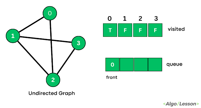
step 1 for bfs traversal
Step 1
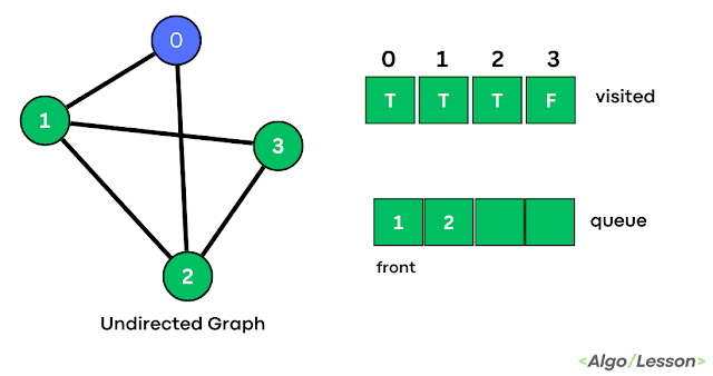
The BFS traversal order of the above graph is starting from vertex 0 so we push the vertex 0 inside the queue and mark that index as visited.
 
step 2 for bfs traversal
Step 2
Pop the front element 0 from the queue and print it. Push the adjacent vertices 1 and 2 inside the queue and then mark them as visited.
step 3 for bfs traversal
Step 3

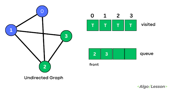
Pop the front element 1 from the queue and print it. Push the adjacent vertices 2 and 3 inside the queue but 2 is already visited so push only 3 and then mark them as visited.
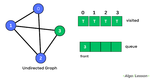
step 4 for bfs traversal
Step 4
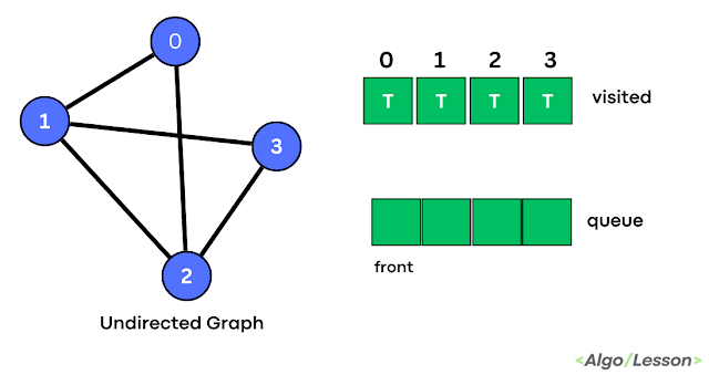
Pop the front element 2 from the queue and print it. Push the adjacent vertices 3 inside the queue but 3 is already visited so nothing to push.
step 5 for bfs traversal
Step 5
Pop the front element 3 from the queue and print it. Push the adjacent vertices if any and mark them as visited. We can observe that we have visited all the vertices of the given graph. Stop the process once the queue is empty.

C++ Code for BFS Traversal Using Queue.

Here is an example of BFS implementation in C++ for an undirected graph represented as an adjacency list:

//C++ Code for BFS Traversal of Undirected Graph
#include <iostream>
#include <vector>
#include <queue>
using namespace std;

//breadth first search of traversal
void bfs(int V, vector<int> adj_list[], int start) {
    vector<bool> visited(V, false);
    queue<int> q;
    visited[start] = true;
    q.push(start);
    while (!q.empty()) {
        int current_vertex = q.front();
        q.pop();
        cout << current_vertex << " ";
        for (auto neighbor : adj_list[current_vertex]) {
            if (!visited[neighbor]) {
                visited[neighbor] = true;
                q.push(neighbor);
            }
        }
    }
}

int main() {
    int V = 4;
    vector<int> adj_list[V];
    adj_list[0] = {1, 2};
    adj_list[1] = {0, 2, 3};
    adj_list[2] = {0, 1, 3};
    adj_list[3] = {1, 2};

    bfs(V, adj_list, 0);

    return 0;
}
Output:
0 1 2 3
  • Time Complexity: O(V + E) where V is the number of vertices and E is the number of edges.
  • Space Complexity: O(V) where one visited array of size V is used to mark visited vertices and one queue to store adjacent vertices while traversing.


BFS Traversal for Disconnected Graph.

The above code for BFS Traversal will not work if the given graph is disconnected. To understand this concept we first have to understand what is disconnected graph.

Disconnected Graph.

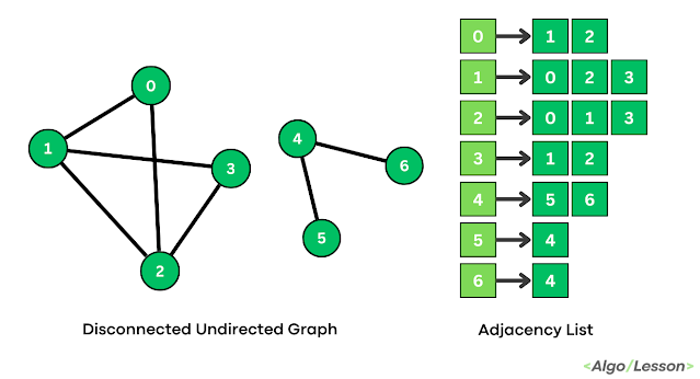
A disconnected graph is a graph in which there is no path between at least two vertices. In other words, a disconnected graph can be split into two or more connected components, where each component contains a group of vertices that are connected to each other but not connected to the vertices in other components.

Example: 
bfs traversal for disconnected graph
Disconnected Graph

We can traverse the disconnected graph by modifying the above BFS code. Below is the C++ code implementation for the BFS traversal of the disconnected graph.

//C++ Code for BFS Traversal of disconnected graph
#include <iostream>
#include <vector>
#include <queue>
using namespace std;

//breadth first search of traversal
void bfs(int V, vector<int> adj_list[], int start, vector<bool> &visited) {
    
    queue<int> q;
    visited[start] = true;
    q.push(start);
    while (!q.empty()) {
        int current_vertex = q.front();
        q.pop();
        cout << current_vertex << " ";
        for (auto neighbor : adj_list[current_vertex]) {
            if (!visited[neighbor]) {
                visited[neighbor] = true;
                q.push(neighbor);
            }
        }
    }
}

int main() {
    int V = 7;
    vector<int> adj_list[V];
    adj_list[0] = {1, 2};
    adj_list[1] = {0, 2, 3};
    adj_list[2] = {0, 1, 3};
    adj_list[3] = {1, 2};
    adj_list[4] = {5, 6};
    adj_list[5] = {4};
    adj_list[6] = {4};

    vector<bool> visited(V, false);
    //for disconnected graph
    for(int i = 0; i < V; i++){
        if(!visited[i]){
            bfs(V, adj_list, i, visited);
        }
    }

    return 0;
}
Output:
0 1 2 3 4 5 6
  • Time Complexity: O(V + E) where V is the number of vertices and E is the number of edges.
  • Space Complexity: O(V) because we are using a visited array of size V and a queue data structure to store adjacent vertices and it is taken at max V size.

Adjacency List Implementation in C++.

In the previous posts, we covered the basics of graph data structure and how we use an adjacency matrix for its representation. Here we are going to learn how to represent graph data structure using Adjacency List.


Adjacency List.

An adjacency list is a way of representing a graph as an array of linked lists, where each vertex has a linked list of its adjacent vertices. In this representation, we create an array of sizes V (V is the number of vertices). Each index of the array will carry a different list which will contain the list of vertices connected to that particular index.


Adjacency List for an Undirected Graph.

In an undirected graph, each edge is bidirectional, meaning that if there's an edge from vertex u to vertex v, there's also an edge from v to u. Therefore, in the adjacency list representation of an undirected graph, we add both u to the adjacency list of v and v to the adjacency list of u.

Example: 

adjacency list in undirected graph
Adjacency List for Undirected Graph

C++ code Implementation of Adjacency List for the above-undirected graph:

//C++ Code for Printing Adjacency List of Undirected Graph
#include <iostream>
#include <vector>
using namespace std;

//Add edges to undirected graph
void addEdge(vector<int> adj[], int u, int v) {
    adj[u].push_back(v);
    adj[v].push_back(u);
}

//printing the adjacency list
void printGraph(vector<int> adj[], int V) {
    for (int v = 0; v < V; ++v) {
        cout << "Adjacency list of vertex " << v << "->";
        for (auto u : adj[v])
            cout << u << " ";
        cout << endl;
    }
}

int main() {
    int V = 4;
    vector<int> adj[V];
    addEdge(adj, 0, 1);
    addEdge(adj, 0, 2);
    addEdge(adj, 1, 2);
    addEdge(adj, 1, 3);
    addEdge(adj, 2, 3);
    printGraph(adj, V);
    return 0;
}
Output:
Adjacency list of vertex 0->1 2
Adjacency list of vertex 1->0 2 3
Adjacency list of vertex 2->0 1 3
Adjacency list of vertex 3->1 2


Adjacency List for a Directed Graph.

In a directed graph, each edge is unidirectional, meaning that there's an edge from vertex u to vertex v, but not necessarily from v to u. Therefore, in the adjacency list representation of a directed graph, we only add v to the adjacency list of u.

Example:

adjacency list of directed graph
Adjacency List for Directed Graph


C++ code Implementation of Adjacency List for the above-directed graph:

//C++ Code for Printing Adjacency List of Directed Graph
#include <iostream>
#include <vector>
using namespace std;

//Add edges to directed graph
void addEdge(vector<int> adj[], int u, int v) {
    adj[u].push_back(v);
}

//printing the adjacency list
void printGraph(vector<int> adj[], int V) {
    for (int v = 0; v < V; ++v) {
        cout << "Adjacency list of vertex " << v << "->";
        for (auto u : adj[v])
            cout << u << " ";
        cout << endl;
    }
}

int main() {
    int V = 4;
    vector<int> adj[V];
    addEdge(adj, 0, 1);
    addEdge(adj, 0, 2);
    addEdge(adj, 1, 2);
    addEdge(adj, 2, 3);
    addEdge(adj, 3, 1);
    printGraph(adj, V);
    return 0;
}
Output:
Adjacency list of vertex 0->1 2
Adjacency list of vertex 1->2
Adjacency list of vertex 2->3
Adjacency list of vertex 3->1

The Adjacency list is an efficient way to represent the graph when the graph is less dense but when the graph is dense we use the Adjacency matrix to represent a graph.

Adjacency Matrix Implementation in C++

We have covered Graph data structure in our previous post and in there, we have learned that graphs can be represented in two different ways, one is Adjacency Matrix and another is Adjacency List. In this post, we are going to learn about the Adjacency Matrix and its implementation for different types of graphs.


Adjacency Matrix.

An adjacency matrix is a way of representing a graph as a matrix of size n x n filled with 0s and 1s, where n is the number of vertices in the graph. The entry in the ith row and jth column of the matrix indicates whether there is an edge from vertex i to vertex j. 


Adjacency Matrix implementation is different for directed and undirected graphs. Let's learn the implementation one by one.


Adjacency Matrix for Undirected Graph.

For a simple undirected graph, the matrix is symmetric around its diagonal, since the edges are bidirectional. It means if there is an edge between vertex A to vertex B then there must be an edge from vertex B to vertex A. 

Note: The diagonal entries in the matrix are always 0 in an undirected graph since there are no self-loops. Also, the matrix is symmetric about its diagonal, so the entry in row i and column j is the same as the entry in row j and column i. (alert-passed)

Example:

adjacency matrix for undirected graph
Adjacency Matrix for Undirected Graph

Below is the C++ code implementation for the Adjacency matrix of an undirected graph.

//C++ code for printing adjacency matrix of undirected graph
#include <iostream>
using namespace std;

const int MAX_SIZE = 100;
int adj_matrix[MAX_SIZE][MAX_SIZE];

int main() {
    // n: number of vertices, m: number of edges
    int n, m;
    cout<<"Enter number of vertices: ";
    cin >> n;
    cout<<"Enter number of edges: ";
    cin >> m;
    
    // initialize adjacency matrix
    for (int i = 0; i < n; ++i) {
        for (int j = 0; j < n; ++j) {
            adj_matrix[i][j] = 0;
        }
    }
    
    cout<< "Add edges to the graph:\n";
    for (int i = 0; i < m; ++i) {
        int u, v;
        cin >> u >> v;
        // since the graph is undirected
        adj_matrix[u][v] = 1;
        adj_matrix[v][u] = 1;
    }
    
    // print adjacency matrix
    cout << "Adjacency matrix:\n";
    for (int i = 0; i < n; ++i) {
        for (int j = 0; j < n; ++j) {
            cout << adj_matrix[i][j] << " ";
        }
        cout << "\n";
    }
    
    return 0;
}
Output:
Enter number of vertices: 4
Enter number of edges: 5
Add edges to the graph:
0 1
0 2
1 2
1 3
2 3
Adjacency matrix:
0 1 1 0
1 0 1 1
1 1 0 1
0 1 1 0


Adjacency Matrix for Directed Graph.

For a directed graph, the matrix is not necessarily symmetric, since the edges are not bidirectional. 

Example:

Adjacency Matrix of Directed Graph
Adjacency Matrix for Directed Graph

Below is the C++ code implementation for the Adjacency matrix of a directed graph.
//C++ code for printing adjacency matrix of directed graph
#include <iostream>
using namespace std;

const int MAX_SIZE = 100;
int adj_matrix[MAX_SIZE][MAX_SIZE];

int main() {
    // n: number of vertices, m: number of edges
    int n, m;
    cout<<"Enter number of vertices: ";
    cin >> n;
    cout<<"Enter number of edges: ";
    cin >> m;
    
    // initialize adjacency matrix
    for (int i = 0; i < n; ++i) {
        for (int j = 0; j < n; ++j) {
            adj_matrix[i][j] = 0;
        }
    }
    
    cout<< "Add edges to the graph:\n";
    for (int i = 0; i < m; ++i) {
        int u, v;
        cin >> u >> v;
        // since the graph is directed
        adj_matrix[u][v] = 1;
    }
    
    // print adjacency matrix
    cout << "Adjacency matrix:\n";
    for (int i = 0; i < n; ++i) {
        for (int j = 0; j < n; ++j) {
            cout << adj_matrix[i][j] << " ";
        }
        cout << "\n";
    }
    
    return 0;
}
Output:
Enter number of vertices: 4
Enter number of edges: 5
Add edges to the graph:
0 1
0 2
1 2
2 3
3 1
Adjacency matrix:
0 1 1 0
0 0 1 0
0 0 0 1
0 1 0 0

Adjacency Matrix is a simple and efficient way to represent a dense graph but we have another method of representation like the Adjacency list when the graph is not dense. 

Difference Between Graph and Tree Data Structure.

Graph and Tree are completely two different data structures and we should handle both differently. Many times we do not know the basic difference between them and here in this post, we are going to discuss some of the important differences between graph and tree data structure.


Graph Data Structure.

A graph is a data structure that is used to represent a collection of interconnected objects, called vertices or nodes, and the connections between them, called edges.

Example:


Tree Data Structure.

A tree is a specific type of graph that is connected and acyclic with a hierarchical structure.

Example:


Difference Between Graph and Tree.

Tree Data Structure Graph Data Structure
A tree is a special type of graph in which any two nodes are connected by exactly one path. A graph, on the other hand, can have multiple paths between two nodes.
Trees have a rooted structure with a single node called the root, from which all other nodes are accessible by a unique path. Graphs do not have a rooted structure.
Trees do not have any cycles. Graphs can have cycles.
In a tree, every node can have at most one parent and multiple children. In a graph, nodes can have multiple parents and children.
Trees are commonly used for hierarchical data structures such as file systems, family trees, and organization charts. Graphs are used for modeling complex relationships and networks such as social networks, transportation systems, and computer networks.
We used In-order, Pre-order, or Post-order traversals to traverse the tree. We used BFS (Breadth-First-Search) and DFS (Depth-First-Search) to traverse the graph.

Conclusion.

A tree is a specific type of graph with a hierarchical structure, no cycles, and a single root node. Graphs, on the other hand, are more general and can have cycles, multiple roots, and complex relationships between nodes.

Types of Graphs in Data Structure.

Graphs are non-linear data structures used to represent interconnected objects called vertices and nodes. A vertex represents a single entity in the graph, such as a person in a social network. An edge represents a connection between two vertices, such as a friendship between two people. We covered graph data structure in our previous post.


Here is the list of some common types of graphs:

1. Undirected Graph.

A graph in which edges have no direction associated with them is called an undirected graph. Example: A network of roads connecting various cities in a country.

Undirected Graph diagram

2. Directed Graph.

A graph in which edges have a direction associated with them is called a directed graph or digraph. Example: A social network where people follow each other on Twitter.

Directed Graph diagram

3. Weighted Graph.

A graph in which edges have weights or costs associated with them is called a weighted graph. Example: A graph representing a road network where the weight of each edge could represent the distance between two cities.

Weighted Graph diagram

4. Complete Graph.

A graph in which every pair of vertices is connected by an edge is called a complete graph. Example: A graph representing a round-robin tournament where every participant plays against another participant exactly once.

Complete Graph diagram

5. Cyclic Graph.

A graph in which all vertices are connected in a cycle is called a cyclic graph. Example: A graph representing a circular arrangement of objects.

Cyclic Graph Diagram

6. Bipartite Graph.

A bipartite graph is a graph in which vertices can be divided into two disjoint sets such that every edge connects a vertex in one set to a vertex in the other set. Example: We have Set X = {A, B, C} and Set Y = {1, 2, 3, 4} and in the graph, the vertices of Set X are only connected with vertices of Set Y and visa-versa.

Bipartite Graph Diagram

7. Tree.

A connected acyclic graph is called a tree. Example: A family tree representing relationships between members of a family.

Tree Diagram

8. Planar Graph.

A graph that can be drawn on a plane without any edges crossing is called a planar graph. Example: A graph representing a geographical map of a city.


9. Sparse Graph.

A graph with few edges compared to the maximum number of edges possible is called a sparse graph. Example: A graph representing a social network where most people are only connected to a few others.


10. Dense Graph.

A graph with many edges compared to the maximum number of edges possible is called a dense graph. Example: A graph representing a road network where most cities are connected to several others.


Graph Data Structure in C++.

A graph is a data structure that is used to represent a collection of interconnected objects, called vertices or nodes, and the connections between them, called edges. 

  • Vertex (or Node): A vertex represents a single entity in the graph, such as a person in a social network or a city in a transportation network.
  • Edge: An edge represents a connection between two vertices, such as a friendship between two people or a road between two cities.

graph data structure

Let's understand graphs through an example, Social networks are a collection of individuals or entities, connected by various relationships or interactions, such as friendships, followings, and likes. 


A social network can be represented using a graph, where each individual or entity is represented as a node, and each relationship or interaction is represented as an edge.


Graph Important Terminology.

  • Directed Graph: A directed graph is a graph in which each edge has a direction associated with it, indicating the flow or direction of the connection between the vertices.
  • Undirected Graph: An undirected graph is a graph in which each edge does not have a direction associated with it, indicating that the connection between the vertices is bidirectional.
  • Weighted Graph: A weighted graph is a graph in which each edge has a weight or cost associated with it, indicating the strength or importance of the connection between the vertices.
  • Degree: The degree of a vertex is the number of edges connected to it. In a directed graph, the degree is further divided into in-degree and out-degree, which represent the number of incoming and outgoing edges, respectively.
  • Path: A path in a graph is a sequence of vertices and edges that connects two vertices. The length of a path is the number of edges in the path.
  • Cycle: A cycle is a path in a graph that starts and ends at the same vertex.
  • Connected Graph: A connected graph is a graph in which there is a path between every pair of vertices.
  • Spanning Tree: A spanning tree is a subset of the edges in a graph that connects all vertices without forming a cycle.


Graph Representation.

There are two common ways to represent a graph data structure: the adjacency list and the adjacency matrix.

Adjacency Matrix.

In the adjacency matrix representation, we use a two-dimensional array for size VxV to represent the edges between vertices. The value at matrix[i][j] represents the weight or existence of the edge between vertices i and j

graph adjacent matrix

C++ Code to Print the Adjacent Matrix of the above graph.
#include <iostream>
using namespace std;

const int MAX_SIZE = 100;
int adj_matrix[MAX_SIZE][MAX_SIZE];

int main() {
    int n, m; // n: number of vertices, m: number of edges
    cin >> n >> m;
    
    // initialize adjacency matrix
    for (int i = 0; i < n; ++i) {
        for (int j = 0; j < n; ++j) {
            adj_matrix[i][j] = 0;
        }
    }
    
    // add edges to the graph
    for (int i = 0; i < m; ++i) {
        int u, v;
        cin >> u >> v;
        // since the graph is undirected
        adj_matrix[u][v] = 1;
        adj_matrix[v][u] = 1;
    }
    
    // print adjacency matrix
    cout << "Adjacency matrix:\n";
    for (int i = 0; i < n; ++i) {
        for (int j = 0; j < n; ++j) {
            cout << adj_matrix[i][j] << " ";
        }
        cout << "\n";
    }
    
    return 0;
}
Output:
5 6
0 1
0 2
0 4
1 4
1 2
2 3
Adjacency matrix:
0 1 1 0 1
1 0 1 0 1
1 1 0 1 0
0 0 1 0 0
1 1 0 0 0


Adjacency List.

In the adjacency list representation, we store each vertex and its neighbors in a dictionary or hash map. The keys of the dictionary represent the vertices, and the values represent the neighboring vertices as a list or set. 

graph adjacency list

C++ Code to Print the Adjacent List of the above graph.
#include <iostream>
#include <vector>
using namespace std;

const int MAX_SIZE = 100;
vector<int> adj_list[MAX_SIZE];

int main() {
    int n, m; // n: number of vertices, m: number of edges
    cin >> n >> m;
    
    // add edges to the graph
    for (int i = 0; i < m; ++i) {
        int u, v;
        cin >> u >> v;
        // since the graph is undirected
        adj_list[u].push_back(v);
        adj_list[v].push_back(u);
    }
    
    // print adjacency list
    cout << "Adjacency list:\n";
    for (int i = 0; i < n; ++i) {
        cout << i << " -> ";
        for (int j = 0; j < adj_list[i].size(); ++j) {
            cout << adj_list[i][j] << " ";
        }
        cout << "\n";
    }
    
    return 0;
}
Output:
5 6
0 1
0 2
0 4
1 2
1 4
2 3
Adjacency list:
0 -> 1 2 4
1 -> 0 2 4
2 -> 0 1 3
3 -> 2
4 -> 0 1

Advantage of Adjacency Matrix and Adjacency List.

The adjacency list is more memory-efficient for sparse graphs (where the number of edges is much less than the number of vertices) and allows for faster iteration over the neighbors of a vertex.(alert-passed)
The adjacency matrix is more efficient for dense graphs (where the number of edges is close to the number of vertices) and allows for constant-time access to the weight or existence of an edge between any two vertices.(alert-passed)

DON'T MISS

Nature, Health, Fitness
© all rights reserved
made with by AlgoLesson