10 Essential Windows Shortcuts Every User Should Know.

Windows Shortcuts

Windows shortcuts are an incredibly powerful and efficient way to navigate and control your PC. They allow you to quickly perform tasks and access features without having to waste time clicking through menus or using a mouse. In this article, we will cover 10 essential Windows shortcuts that every user should know.


Windows Key + D

The Windows Key + D shortcut will quickly minimize all open windows and take you straight to your desktop. This is a handy shortcut when you need to access files or folders on your desktop or when you want to quickly switch between applications.


Windows Key + E

The Windows Key + E shortcut will launch Windows Explorer, giving you quick access to all of your files and folders. This is a great way to quickly browse through your files and find what you need without having to open up individual folders.


Windows Key + L

The Windows Key + L shortcut is a quick way to lock your computer when you need to step away from your desk. This is a useful shortcut if you work in an office or public space and want to keep your computer secure.


Windows Key + R

The Windows Key + R shortcut will open the Run dialog box, allowing you to quickly launch programs, files, and folders by typing in their names. This is a great way to quickly access programs or files that you use frequently.


Ctrl + C / Ctrl + X / Ctrl + V

These are the three most common keyboard shortcuts used for copying, cutting, and pasting. Simply select the text or files you want to copy or cut, use Ctrl + C or Ctrl + X, then navigate to where you want to paste the text or files and use Ctrl + V.


Windows Key + Tab

The Windows Key + Tab shortcut is a great way to quickly switch between open applications. It works similarly to Alt + Tab, but with a more visual interface that allows you to see all of your open windows at once.


Ctrl + Z / Ctrl + Y

These shortcuts are used for undoing and redoing actions. If you make a mistake, use Ctrl + Z to undo your last action. If you change your mind and want to redo your action, use Ctrl + Y.


Windows Key + I

The Windows Key + I shortcut will open the Settings app, which is the central hub for managing your Windows settings. From here, you can manage everything from your display settings to your security and privacy settings.


Alt + F4

The Alt + F4 shortcut is a quick way to close an open application. It is a great way to quickly shut down a program that has frozen or is not responding.


Ctrl + Shift + Esc

The Ctrl + Shift + Esc shortcut will open the Task Manager, which is a powerful tool for managing and monitoring your system processes. You can use the Task Manager to see which applications are using the most resources and to close any programs that are causing problems.


Conclusion.

These 10 essential Windows shortcuts will help you navigate and control your PC more efficiently. By using these shortcuts, you can save time and streamline your workflow, making you a more productive and efficient computer user.

Swap Two Numbers in Java.

We can swap two numbers in Java with multiple approaches and in this article, we are going to discuss all those approaches in detail with code.


Approach 1: Using a third variable

In this approach, we use a third variable to swap the values of the two variables.


Java Example Code:

int a = 10;
int b = 20;
int temp;

temp = a;
a = b;
b = temp;

System.out.println("a = " + a); // Output: a = 20
System.out.println("b = " + b); // Output: b = 10

Approach 2: Using arithmetic operations

In this approach, we can use arithmetic operations like addition, subtraction, multiplication, and division to swap the values of the two variables.

Java Example Code:
int a = 10;
int b = 20;

a = a + b; // a = 30
b = a - b; // b = 10
a = a - b; // a = 20

System.out.println("a = " + a); // Output: a = 20
System.out.println("b = " + b); // Output: b = 10

Approach 3: Using the XOR operator

In this approach, we can use the XOR (^) operator to swap the values of the two variables.

Java Example Code:

int a = 10;
int b = 20;

a = a ^ b; // a = 30 (11110)
b = a ^ b; // b = 10 (01010)
a = a ^ b; // a = 20 (10100)

System.out.println("a = " + a); // Output: a = 20
System.out.println("b = " + b); // Output: b = 10
All these approaches have the same time complexity of O(1) as they take constant time to swap the values of two variables. (alert-success)

Difference Between Default and Parameterless Constructor in C++

Constructor is an important concept to understand in Object Oriented Programming and we have many constructors like default, parameterized, and copy constructors. Many get confused that is there any difference between a default constructor and a parameterless constructor. 


In C++, a default constructor and a parameterless constructor are similar in that they both create objects without requiring any arguments. However, there is a subtle difference between the two.


Default Constructor.

A default constructor is a constructor that the compiler generates automatically if no constructor is defined explicitly for a class. The default constructor has no parameters and initializes the data members of the object to their default values (which are typically zero for numeric types and null or empty for pointers and strings).

Example:

class MyClass {
public:
    MyClass() {
        // Default constructor
        // Initialize data members with default values
    }
};


Parameterless Constructor.

A parameterless constructor, on the other hand, is a constructor that is defined explicitly by the programmer and has no parameters. The programmer can define the behavior of the parameterless constructor to initialize the object in any way they see fit.

Example:

class MyClass {
public:
    MyClass(int value) {
        // Parameterized constructor
        // Initialize data members with the provided 'value'
    }
};

Round Up the Result of Integer Division in C++.

In C++, the integer division of two integers produces a result that is truncated toward zero. For example, if we divide 5 by 2, the result would be 2 instead of 2.5, because the decimal part is truncated. However, there are times when we want the result of integer division to be rounded up to the nearest integer. 


Round Up Integer Division using Formula.

Suppose we want to compute the result of integer division a/b and round it up to the nearest integer. We can do this using the following formula:


int result = (a + b - 1) / b;

The idea behind this formula is that we add b-1 to the numerator, which ensures that the division result is always rounded up. 
Example:
int a = 5;
int b = 2;
int result = (a + b - 1) / b;
result is 3, not 2

In this example, the numerator (a+b-1) is 6, and the denominator (b) is 2. The result of the division is therefore 3, which is the closest integer to 2.5, the exact result of the division.
Note: This formula works only for positive integers. If a or b can be negative, you should use a different formula. (alert-passed)

C++ program that demonstrates how to round up the result of integer division:

//C++ code to round up integer division
#include <iostream>
using namespace std;

int main() {
    int a = 5;
    int b = 2;
    int result = (a + b - 1) / b;
    cout << "The result of " << a << " / " << b << " rounded up is " << result << endl;
    return 0;
}
Output:
The result of 5 / 2 rounded up is 3

Round Up Using Ceil() Function.

C++, you can use the ceil() function from the <cmath> header to round up a floating-point value to the nearest integer. However, it's important to note that ceil() works with floating-point values, not with the result of integer division.
Note: If you want to round up the result of integer division, you would need to convert the integers to floating-point values before using ceil() (alert-success)

C++ Code Implementation:

//C++ code to round up integer uisng ceil fun
#include <iostream>
#include <cmath>
using namespace std;

int main() {
    int a = 5;
    int b = 2;
    double result = ceil(static_cast<double>(a) / b);
    cout << "The result of " << a << " / " << b << " rounded up is " << result << endl;
    return 0;
}
Output:
The result of 5 / 2 rounded up is 3

Depth First Search for Graph in C++.

Depth First Search (DFS) is a graph traversal algorithm that explores a graph by visiting as far as possible along each branch before backtracking. It starts from a given source vertex and recursively explores all of its neighbors, marking each vertex as visited as it traverses the graph. Once it reaches the end of a branch, it backtracks to the last unexplored vertex and continues the search.


Algorithm for Depth First Search.

  • Step 1: Create a visited array and initialize it to false.
  • Step 2: Initialize a stack and push the source vertex onto it.
  • Step 3: While the stack is not empty, do the following:
  • a. Pop a vertex from the stack.
  • b. If the vertex has not been visited, mark it as visited and do the following:
  • i. Process the vertex (e.g., print its value).
  • ii. Get its neighbors and push them onto the stack.
  • Step 4: Repeat step 3 until the stack is empty.

Example with Illustration.

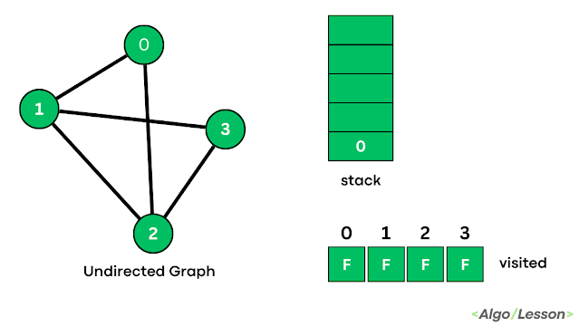
depth first search step 1
Step 1

We have one stack to traverse all vertices and a visited array to mark visited vertices. Push the starting vertex 0 in the stack as the initial condition. 

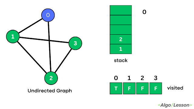
depth first search step 2
Step 2
Pop the top element of the stack that is 0 and mark that index as visited in the visited array and print it. Push all other neighbor vertices of 0 inside the stack if already not visited.
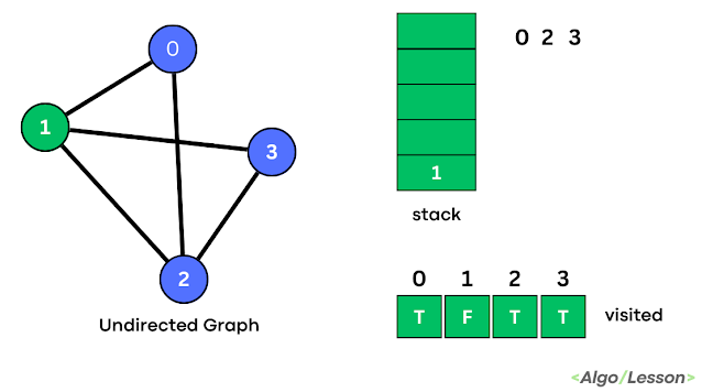
depth first search step 3
Step 3

Pop the top element of the stack that is 2 and mark that index as visited in the visited array and print it. Push all other neighbor vertices of 2 inside the stack if already not visited.
depth first search step 4
Step 4
Pop the top element of the stack that is 3 and mark that index as visited in the visited array and print it. Push all other neighbor vertices of 3 inside the stack if already not visited.
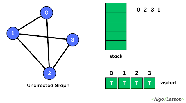
depth first search step 5
Step 5
Pop the top element of the stack that is 1 and mark that index as visited in the visited array and print it. Push all other neighbor vertices of 3 inside the stack if already not visited. Here the stack becomes empty which means traversal is complete.

C++ code for DFS (Depth First Search) Traversal using Stack.

//C++ code implementation for DFS Traversal of graph using Stack
#include <iostream>
#include <vector>
#include <stack>
using namespace std;

//function for dfs
void DFS(int V, vector<int> graph[], int start, vector<bool>& visited) {
    stack<int> s;
    s.push(start);

    while (!s.empty()) {
        int v = s.top();
        s.pop();

        if (!visited[v]) {
            visited[v] = true;
            cout << v << " ";

            for (int u : graph[v]) {
                s.push(u);
            }
        }
    }
}

int main() {
    int V = 4;
    vector<int> graph[V];
    graph[0] = {1, 2};
    graph[1] = {0, 2, 3};
    graph[2] = {0, 1, 3};
    graph[3] = {1, 2};

    vector<bool> visited(V, false);
    DFS(V, graph, 0, visited);
    return 0;
}
Output:
0 2 3 1
  • Time Complexity: O(V + E) where V is the number of vertices and E is the number of Edges. Each vertex and each edge is explored exactly once.
  • Space Complexity: O(V + E) as it uses a stack to keep track of vertices and an array to mark visited vertices. In the worst case, the stack will store all vertices of the longest path, which is the maximum the maximum depth of the recursion.


Algorithm for Depth First Search (Recursive).

  • Step 1: Create a visited array and initialize it to false.
  • Step 2: Call the DFS function with the starting vertex as the argument.
  • Step 3: In the DFS function, mark the current vertex as visited and process it (e.g., print its value).
  • Step 4: For each unvisited neighbor of the current vertex, recursively call the DFS function with the neighbor as the argument.
C++ code for DFS (Depth First Search) Traversal using Recursion:

//C++ code implementation for DFS Traversal of graph using Recursion
#include <iostream>
#include <vector>
#include <stack>
using namespace std;

//function for dfs
void DFS(int V, vector<int> graph[], int start, vector<bool>& visited) {
    visited[start] = true;
    cout << start << " ";

    for (int u : graph[start]) {
        if (!visited[u]) {
            DFS(V, graph, u, visited);
        }
    }
}

int main() {
    int V = 4;
    vector<int> graph[V];
    graph[0] = {1, 2};
    graph[1] = {0, 2, 3};
    graph[2] = {0, 1, 3};
    graph[3] = {1, 2};

    vector<bool> visited(V, false);
    DFS(V, graph, 0, visited);
    return 0;
}
Output:
0 1 2 3
  • Time Complexity: O(V + E) where V is the number of vertices and E is the number of Edges.
  • Space Complexity: O(V) as an array to mark visited vertices. The maximum depth of the recursion is the number of vertices.

Breadth First Search (BFS) for Graph in C++

Breadth First Search (BFS) is a graph traversal algorithm that visits all the vertices of a graph in breadth-first order, meaning that it visits all the vertices at the same level before moving on to the next level. The algorithm uses a queue data structure to keep track of the vertices that need to be visited.


How BFS for Graph is different from BFS for Tree Data structure?

The main difference between the graph and the tree BFS traversal is that a tree cannot contain cycles but a graph can contain cycles. To avoid visiting the same vertex again and again we use a boolean visited array to mark the visited vertices.


If we don't mark the visited vertices, the algorithm may revisit vertices that have already been explored and get stuck in an infinite loop. This is especially true in the case of cycles, where a BFS traversal without marking visited vertices could result in an infinite loop.


Algorithm of Breadth First Search:

  • Step 1: Create a queue data structure and add the starting vertex to the queue.
  • Step 2: While the queue is not empty:
  • Step 3: Dequeue the vertex at the front of the queue and mark it as visited.
  • Step 4: Visit all the unvisited neighbors of the dequeued vertex and add them to the queue.
  • Step 5: If all the vertices have been visited, the algorithm is complete.

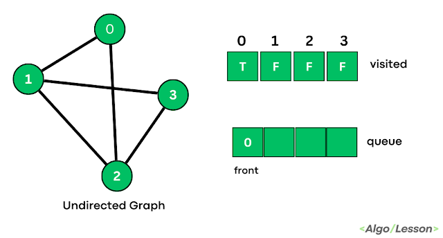
Example with Illustration.

step 1 for bfs traversal
Step 1
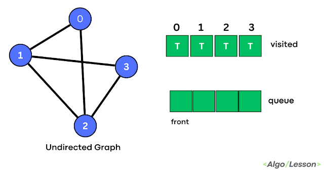
The BFS traversal order of the above graph is starting from vertex 0 so we push the vertex 0 inside the queue and mark that index as visited.
 
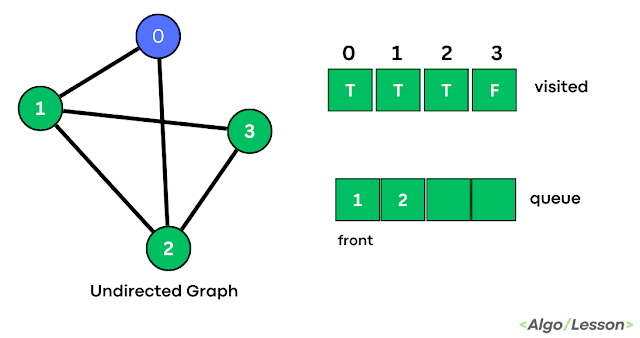
step 2 for bfs traversal
Step 2
Pop the front element 0 from the queue and print it. Push the adjacent vertices 1 and 2 inside the queue and then mark them as visited.
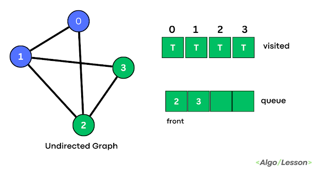
step 3 for bfs traversal
Step 3

Pop the front element 1 from the queue and print it. Push the adjacent vertices 2 and 3 inside the queue but 2 is already visited so push only 3 and then mark them as visited.
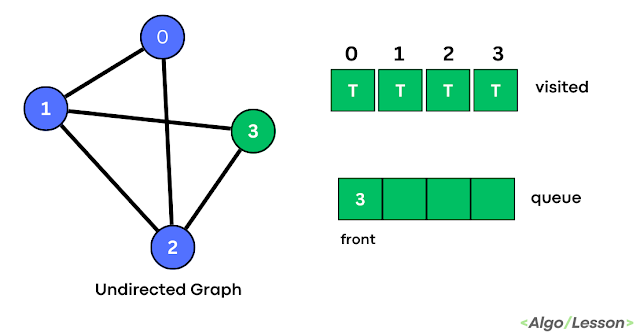
step 4 for bfs traversal
Step 4
Pop the front element 2 from the queue and print it. Push the adjacent vertices 3 inside the queue but 3 is already visited so nothing to push.
step 5 for bfs traversal
Step 5
Pop the front element 3 from the queue and print it. Push the adjacent vertices if any and mark them as visited. We can observe that we have visited all the vertices of the given graph. Stop the process once the queue is empty.

C++ Code for BFS Traversal Using Queue.

Here is an example of BFS implementation in C++ for an undirected graph represented as an adjacency list:

//C++ Code for BFS Traversal of Undirected Graph
#include <iostream>
#include <vector>
#include <queue>
using namespace std;

//breadth first search of traversal
void bfs(int V, vector<int> adj_list[], int start) {
    vector<bool> visited(V, false);
    queue<int> q;
    visited[start] = true;
    q.push(start);
    while (!q.empty()) {
        int current_vertex = q.front();
        q.pop();
        cout << current_vertex << " ";
        for (auto neighbor : adj_list[current_vertex]) {
            if (!visited[neighbor]) {
                visited[neighbor] = true;
                q.push(neighbor);
            }
        }
    }
}

int main() {
    int V = 4;
    vector<int> adj_list[V];
    adj_list[0] = {1, 2};
    adj_list[1] = {0, 2, 3};
    adj_list[2] = {0, 1, 3};
    adj_list[3] = {1, 2};

    bfs(V, adj_list, 0);

    return 0;
}
Output:
0 1 2 3
  • Time Complexity: O(V + E) where V is the number of vertices and E is the number of edges.
  • Space Complexity: O(V) where one visited array of size V is used to mark visited vertices and one queue to store adjacent vertices while traversing.


BFS Traversal for Disconnected Graph.

The above code for BFS Traversal will not work if the given graph is disconnected. To understand this concept we first have to understand what is disconnected graph.

Disconnected Graph.

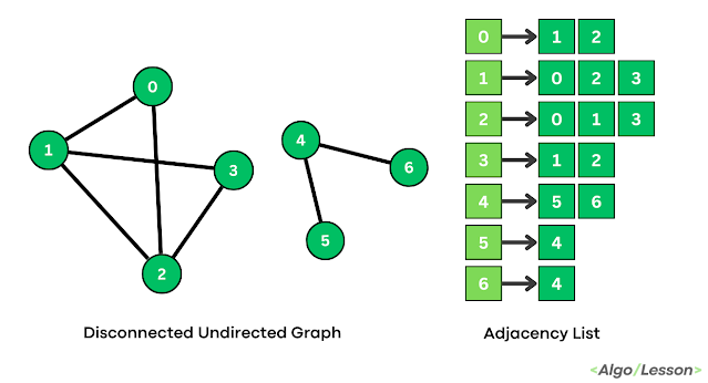
A disconnected graph is a graph in which there is no path between at least two vertices. In other words, a disconnected graph can be split into two or more connected components, where each component contains a group of vertices that are connected to each other but not connected to the vertices in other components.

Example: 
bfs traversal for disconnected graph
Disconnected Graph

We can traverse the disconnected graph by modifying the above BFS code. Below is the C++ code implementation for the BFS traversal of the disconnected graph.

//C++ Code for BFS Traversal of disconnected graph
#include <iostream>
#include <vector>
#include <queue>
using namespace std;

//breadth first search of traversal
void bfs(int V, vector<int> adj_list[], int start, vector<bool> &visited) {
    
    queue<int> q;
    visited[start] = true;
    q.push(start);
    while (!q.empty()) {
        int current_vertex = q.front();
        q.pop();
        cout << current_vertex << " ";
        for (auto neighbor : adj_list[current_vertex]) {
            if (!visited[neighbor]) {
                visited[neighbor] = true;
                q.push(neighbor);
            }
        }
    }
}

int main() {
    int V = 7;
    vector<int> adj_list[V];
    adj_list[0] = {1, 2};
    adj_list[1] = {0, 2, 3};
    adj_list[2] = {0, 1, 3};
    adj_list[3] = {1, 2};
    adj_list[4] = {5, 6};
    adj_list[5] = {4};
    adj_list[6] = {4};

    vector<bool> visited(V, false);
    //for disconnected graph
    for(int i = 0; i < V; i++){
        if(!visited[i]){
            bfs(V, adj_list, i, visited);
        }
    }

    return 0;
}
Output:
0 1 2 3 4 5 6
  • Time Complexity: O(V + E) where V is the number of vertices and E is the number of edges.
  • Space Complexity: O(V) because we are using a visited array of size V and a queue data structure to store adjacent vertices and it is taken at max V size.

Adjacency List Implementation in C++.

In the previous posts, we covered the basics of graph data structure and how we use an adjacency matrix for its representation. Here we are going to learn how to represent graph data structure using Adjacency List.


Adjacency List.

An adjacency list is a way of representing a graph as an array of linked lists, where each vertex has a linked list of its adjacent vertices. In this representation, we create an array of sizes V (V is the number of vertices). Each index of the array will carry a different list which will contain the list of vertices connected to that particular index.


Adjacency List for an Undirected Graph.

In an undirected graph, each edge is bidirectional, meaning that if there's an edge from vertex u to vertex v, there's also an edge from v to u. Therefore, in the adjacency list representation of an undirected graph, we add both u to the adjacency list of v and v to the adjacency list of u.

Example: 

adjacency list in undirected graph
Adjacency List for Undirected Graph

C++ code Implementation of Adjacency List for the above-undirected graph:

//C++ Code for Printing Adjacency List of Undirected Graph
#include <iostream>
#include <vector>
using namespace std;

//Add edges to undirected graph
void addEdge(vector<int> adj[], int u, int v) {
    adj[u].push_back(v);
    adj[v].push_back(u);
}

//printing the adjacency list
void printGraph(vector<int> adj[], int V) {
    for (int v = 0; v < V; ++v) {
        cout << "Adjacency list of vertex " << v << "->";
        for (auto u : adj[v])
            cout << u << " ";
        cout << endl;
    }
}

int main() {
    int V = 4;
    vector<int> adj[V];
    addEdge(adj, 0, 1);
    addEdge(adj, 0, 2);
    addEdge(adj, 1, 2);
    addEdge(adj, 1, 3);
    addEdge(adj, 2, 3);
    printGraph(adj, V);
    return 0;
}
Output:
Adjacency list of vertex 0->1 2
Adjacency list of vertex 1->0 2 3
Adjacency list of vertex 2->0 1 3
Adjacency list of vertex 3->1 2


Adjacency List for a Directed Graph.

In a directed graph, each edge is unidirectional, meaning that there's an edge from vertex u to vertex v, but not necessarily from v to u. Therefore, in the adjacency list representation of a directed graph, we only add v to the adjacency list of u.

Example:

adjacency list of directed graph
Adjacency List for Directed Graph


C++ code Implementation of Adjacency List for the above-directed graph:

//C++ Code for Printing Adjacency List of Directed Graph
#include <iostream>
#include <vector>
using namespace std;

//Add edges to directed graph
void addEdge(vector<int> adj[], int u, int v) {
    adj[u].push_back(v);
}

//printing the adjacency list
void printGraph(vector<int> adj[], int V) {
    for (int v = 0; v < V; ++v) {
        cout << "Adjacency list of vertex " << v << "->";
        for (auto u : adj[v])
            cout << u << " ";
        cout << endl;
    }
}

int main() {
    int V = 4;
    vector<int> adj[V];
    addEdge(adj, 0, 1);
    addEdge(adj, 0, 2);
    addEdge(adj, 1, 2);
    addEdge(adj, 2, 3);
    addEdge(adj, 3, 1);
    printGraph(adj, V);
    return 0;
}
Output:
Adjacency list of vertex 0->1 2
Adjacency list of vertex 1->2
Adjacency list of vertex 2->3
Adjacency list of vertex 3->1

The Adjacency list is an efficient way to represent the graph when the graph is less dense but when the graph is dense we use the Adjacency matrix to represent a graph.

DON'T MISS

Nature, Health, Fitness
© all rights reserved
made with by AlgoLesson